Audio Visualizers in ISF
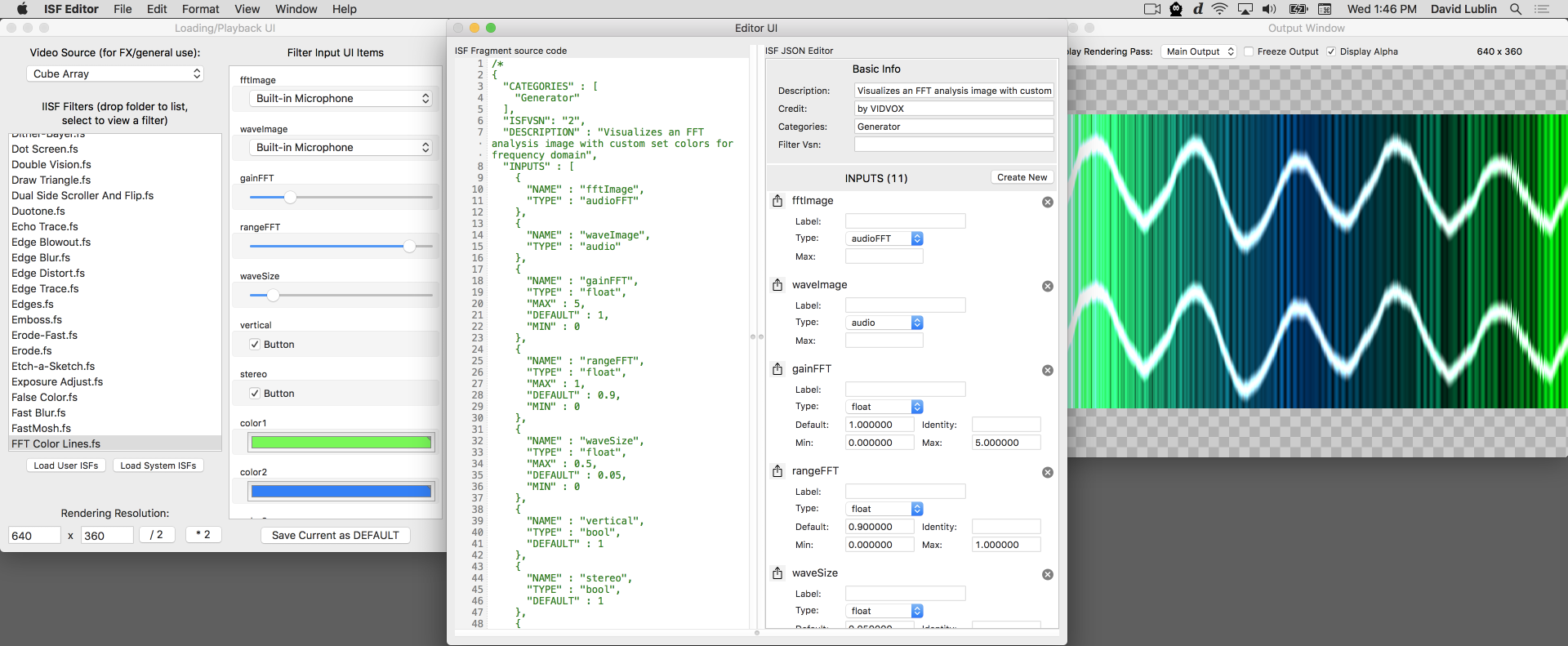 Shader with raw audio and FFT waveform inputs in the ISF Editor.
 Though GLSL as a language has no concept of sound data, many developers have found ways to writes audio-visualizers by converting audio into a format that can be passed to shaders. As one of its extensions to the language, ISF includes a standard way for host software to pass in audio waveforms and FFT information for this purpose.
In this chapter we will discuss:
- How to declare audio waveform inputs for shaders in ISF.
- How to create a basic audio waveform visualizer with ISF.
- The basic idea of an audio FFT.
- How to declare audio FFT inputs for shaders in ISF.
- How to create a basic audio FFT histogram visualizer with ISF.
This chapter includes examples from the ISF Test/Tutorial filters.
For an example of audio waveforms and FFTs used in a host application see the VDMX tutorial on visualizing audio fft and waveforms.
Audio Waveforms in ISF
One of the ways that ISF extends GLSL is by providing a convention for working with audio waveform data. The technique that ISF uses for passing sound information into shaders is for the host application to convert the desired raw audio samples into image data that can be accessed like any other image input.
How audio is stored in images in ISF
Within ISF, audio data packed into images follow the following conventions:
- The width of the image is the number of provided audio samples.
- The height is the number of audio channels.
- The first audio sample temporally corresponds to the first horizontal pixel column (x = 0) in the image.
- The first audio channel corresponds to the first vertical pixel row (y = 0) in the image.
- The rgb channels for each pixel will call contain the same value, representing the amplitude of the signal at the sample time, centered around 0.5. In other words, this will be a grayscale image.
- When possible, the host application may provide 32-bit floating point values instead of 8-bit data.
Declaring audio inputs in ISF
Like with other variables and images that connect our shaders to the host application, for audio we will be adding elements to the INPUTS section of our JSON blob.
To declare an "audio" input in the ISF JSON, there are a two required attributes (TYPE and NAME) and additional optional attributes that can be provided.
- The
TYPEattribute must be set to the string "audio" which specifies that the input will be sent audio waveform data from an audio source. - Like with other inputs, you must provide a
NAMEattribute that contains a unique string that will be used to reference the provided image data in the GLSL code. - "audio"-type inputs support the use of the
MAXkey- but in this context,MAXspecifies the number of samples that the shader wants to receive. This key is optional- ifMAXis not defined then the shader will receive audio data with the number of samples that were provided natively. For example, if theMAXof an "audio"-type input is defined as 1, the resulting 1-pixel-wide image is going to accurately convey the "total volume" of the audio wave; if you want a 4-column FFT graph, specify aMAXof 4 on an "audioFFT"-type input, etc. - As with other elements you can include a custom
LABELattribute that contains a string with a human readable name for the attribute.
An example audio waveform visualizer
From the "ISF tests+tutorials" is this simple audio visualizer shader. In addition to the declared waveImage audio input is an options for setting the wave size and output display style called waveSize.
/*
{
  "CATEGORIES" : [
    "Generator"
  ],
  "DESCRIPTION" : "Visualizes an audio waveform image",
  "INPUTS" : [
    {
      "NAME" : "waveImage",
      "TYPE" : "audio"
    },
    {
      "NAME" : "waveSize",
      "TYPE" : "float",
      "MAX" : 0.5,
      "DEFAULT" : 0.05,
      "MIN" : 0
    }
  ],
  "CREDIT" : "by VIDVOX"
}
*/

void main() {
	//	just grab the first audio channel here
	float		channel = 0.0;

	//	get the location of this pixel
	vec2		loc = isf_FragNormCoord;

	//	though not needed here, note the IMG_SIZE function can be used to get the dimensions of the audio image
	//vec2		audioImgSize = IMG_SIZE(waveImage);

	vec2		waveLoc = vec2(loc.x,channel);
	vec4		wave = IMG_NORM_PIXEL(waveImage, waveLoc);
	vec4		waveAdd = (1.0 - smoothstep(0.0, waveSize, abs(wave - loc.y)));
	gl_FragColor = waveAdd;
}
In the code section for this basic example, the channel to visualizer is set to look at just the first audio channel. In more complex setups you may want to add a selection menu that allows you to pick an individual channel, or write a for loop that iterates over each channel, or you may want to create a visualizer that handles multi-channel audio in some other fashion.
Next we get the location of current pixel, in its normalized (0.0 to 1.0) format. For this shader we will be stretching the raw audio waveform, regardless of how many pixels it is, across the entire width of the output image, so the normalized location is ideal because it can be directly fed into the IMG_NORM_PIXEL function without any additional scaling.
Once the sample value for this particular x coordinate is looked up, the smoothstep() function is used along with the waveSize to see if the y coordinate of the current pixel is within range of the audio sample value.
Audio FFT in ISF
What are Audio FFTs?
FFT is short for "Fast Fourier Transform" which doesn't tell you much about what they do. What we can take away from the name is that they are fast way to transform something and the person that came up with the idea of it was probably named Fourier.
In general usage, FFTs rely on the idea that if you take a snapshot of any stream of data that happens "over time" (also known as occurring "in the time domain") it can be represented as a single function that is a combination of sine waves with different amplitudes and frequencies added together.
That is to say, for any set of 1024 numbers, you can create a function that is made up of 512 amplitude and frequency values such that: y(t) = a0 * sin(f0TIME) + a1 * sin(f1TIME) + ... + a511 * sin(f511 * TIME);
This concept is particularly useful when working with audio waveforms, as FFTs will tell use the amount of energy within a specific frequency range. Each frequency section within the FFT is known as an "FFT bin" and the last frequency will be half the sample rate.
Though it is interesting to learn the low level math behind how FFTs work (and how to compute them by hand), in practical use this is one area where computers are our best friends - to get an FFT from our data, all we have to do is ask politely.
Declaring Audio FFT inputs in ISF
Like with receiving raw audio data, FFTs are declared as part of the INPUTS section of the JSON blob and provided to the code as an image.
Within ISF, audio FFT data packed into images follow the following conventions:
- The width of the image is the number of provided frequency bins. Typically this image will be a power of two in width (128, 256, 512, 1024, etc) and with the final bin representing the "Nyquist frequency" at the current sample rate.
- The height is the number of audio channels.
- The first frequency bin temporally corresponds to the first horizontal pixel column (x = 0) in the image.
- The first audio channel corresponds to the first vertical pixel row (y = 0) in the image.
- The rgb channels for each pixel will call contain the same value, representing the amplitude of the frequency bin during this time snapshot. In other words, this will be a grayscale image.
- When possible, the host application may provide 32-bit floating point values instead of 8-bit data.
To declare an "audioFFT" input in the ISF JSON, there are a two required attributes (TYPE and NAME) and additional optional attributes that can be provided.
- The
TYPEattribute must be set to the string "audioFFT" which specifies that the input will be sent audio waveform data from an audio source. - Like with other inputs, you must provide a
NAMEattribute that contains a unique string that will be used to reference the provided image data in the GLSL code. - "audioFFT"-type inputs support the use of the
MAXkey- but in this context,MAXspecifies the number of samples that the shader wants to receive. This key is optional- ifMAXis not defined then the shader will receive audio data with the number of samples that were provided natively. For example, if theMAXof an "audio"-type input is defined as 1, the resulting 1-pixel-wide image is going to accurately convey the "total volume" of the audio wave; if you want a 4-column FFT graph, specify aMAXof 4 on an "audioFFT"-type input, etc. - As with other elements you can include a custom
LABELattribute that contains a string with a human readable name for the attribute.
An example Audio FFT visualizer
From the ISF tests+tutorials collection is this demonstration of using FFTs. Along with the audioFFT element in the INPUTS portion of the JSON blob, several other uniform variables are declared for adjusting the gain, display range and coloring of the output.
/*{
	"DESCRIPTION": "Visualizes an FFT analysis image with custom set colors for frequency domain",
	"CREDIT": "by VIDVOX",
	"ISFVSN": "2",
	"CATEGORIES": [
		"Generator"
	],
	"INPUTS": [
		{
			"NAME": "fftImage",
			"TYPE": "audioFFT"
		},
		{
			"NAME": "strokeSize",
			"TYPE": "float",
			"MIN": 0.0,
			"MAX": 0.25,
			"DEFAULT": 0.01
		},
		{
			"NAME": "gain",
			"TYPE": "float",
			"MIN": 1.0,
			"MAX": 5.0,
			"DEFAULT": 1.0
		},
		{
			"NAME": "minRange",
			"TYPE": "float",
			"MIN": 0.0,
			"MAX": 1.0,
			"DEFAULT": 0.0
		},
		{
			"NAME": "maxRange",
			"TYPE": "float",
			"MIN": 0.0,
			"MAX": 1.0,
			"DEFAULT": 0.9
		},
		{
			"NAME": "topColor",
			"TYPE": "color",
			"DEFAULT": [
				0.0,
				0.0,
				0.0,
				0.0
			]
		},
		{
			"NAME": "bottomColor",
			"TYPE": "color",
			"DEFAULT": [
				0.0,
				0.5,
				0.9,
				1.0
			]
		},
		{
			"NAME": "strokeColor",
			"TYPE": "color",
			"DEFAULT": [
				0.25,
				0.25,
				0.25,
				1.0
			]
		}
	]
}*/


void main() {

	vec2 loc = isf_FragNormCoord;

	loc.x = loc.x * abs(maxRange - minRange) + minRange;

	vec4 fft = IMG_NORM_PIXEL(fftImage, vec2(loc.x,0.5));
	float fftVal = gain * (fft.r + fft.g + fft.b) / 3.0;
	if (loc.y > fftVal)
		fft = topColor;
	else
		fft = bottomColor;
	if ((strokeSize > 0.0) && (abs(fftVal - loc.y) < strokeSize))	{
		fft = mix(strokeColor, fft, abs(fftVal - loc.y) / strokeSize);
	}

	gl_FragColor = fft;
}
Like with the audio waveform example, the IMG_NORM_PIXEL function is used to retrieve the FFT results. In this code, before the pixel lookup happens, the maxRange and minRange uniform variables are used to adjust the range of values that will be read from the fftImage.
After that the color of the output pixel varies depending on the result from the FFT for the observed bin and the y position of the loc variable. If the current pixel's y position is within strokeSize of the fftVal, the output is mixed with the stroke color.
An example Audio FFT Spectrogram visualizer
As a final example in this chapter we will look at a shader that combines this new concept of audio FFTs with other powerful capabilities in ISF, the ability to store persistent buffers and perform multiple render passes. This will enable us to not just look at the current FFT snapshot, we can store and display multiple FFTs over time.
If we take our FFT data slices and visualize them over time, we are essentially creating what is known as a Spectrogram and you may have seen them before, as they are widely used in the arts, sciences and even show up from time to time in pop-culture. Like FFTs themselves, they can represent all kinds of data and one very common use case is audio.
One particularly cool usage of this is from Aphex Twin in the song "Equation" where an image of a face is essentially encoded in the music, such that when you create a spectrogram from the FFT, the face image is revealed:
Here is the code for making an audio FFT Spectrogram in ISF. Note how we are making use of audioFFT inputs, multiple shader passes and persistent buffers. Like with the previous FFT example there are added inputs for controlling the coloring of the output display. There is also an option to reset the persistent buffer via the clear event.
/*{
	"DESCRIPTION": "Buffers the incoming FFTs for timed display",
	"CREDIT": "by VIDVOX",
	"ISFVSN": "2",
	"CATEGORIES": [
		"Generator"
	],
	"INPUTS": [
		{
			"NAME": "fftImage",
			"TYPE": "audioFFT"
		},
		{
			"NAME": "clear",
			"TYPE": "event"
		},
		{
			"NAME": "gain",
			"TYPE": "float",
			"MIN": 0.0,
			"MAX": 2.0,
			"DEFAULT":1.0
		},
		{
			"NAME": "range",
			"TYPE": "float",
			"MIN": 0.0,
			"MAX": 1.0,
			"DEFAULT": 1.0
		},
		{
			"NAME": "axis_scale",
			"TYPE": "float",
			"MIN": 1.0,
			"MAX": 6.0,
			"DEFAULT": 1.25
		},
		{
			"NAME": "lumaMode",
			"TYPE": "bool",
			"DEFAULT": 0.0
		},
		{
			"NAME": "color1",
			"TYPE": "color",
			"DEFAULT": [
				0.0,
				0.5,
				1.0,
				1.0
			]
		},
		{
			"NAME": "color2",
			"TYPE": "color",
			"DEFAULT": [
				1.0,
				0.0,
				0.0,
				1.0
			]
		},
		{
			"NAME": "color3",
			"TYPE": "color",
			"DEFAULT": [
				0.0,
				1.0,
				0.0,
				1.0
			]
		}
	],
	"PASSES": [
		{
			"TARGET": "fftValues",
			"DESCRIPTION": "This buffer stores all of the previous fft values",
			"HEIGHT": "512",
			"FLOAT": true,
			"PERSISTENT": true
		},
		{

		}
	]

}*/

void main()
{
	//    first pass- read the value from the fft image, store it in the "fftValues" persistent buffer
	if (PASSINDEX==0)    {
		//    the first column of pixels is copied from the newly received fft image
		if (clear)	{
			gl_FragColor = vec4(0.0);
		}
		else if (gl_FragCoord.x<1.0)    {
			vec2		loc = vec2(isf_FragNormCoord.y, isf_FragNormCoord.x);
			vec4		rawColor = IMG_NORM_PIXEL(fftImage, loc);
			gl_FragColor = rawColor;
		}
		//    all other columns of pixels come from the "fftValues" persistent buffer (we're scrolling)
		else    {
			gl_FragColor = IMG_PIXEL(fftValues, vec2(gl_FragCoord.x-1.0, gl_FragCoord.y));
		}
	}
	//    second pass- read from the buffer of raw values, apply gain/range and colors
	else if (PASSINDEX==1)    {
		vec2		loc = vec2(isf_FragNormCoord.x, pow(isf_FragNormCoord.y*range, axis_scale));
		vec4		rawColor = IMG_NORM_PIXEL(fftValues, loc);

		rawColor = rawColor * vec4(gain);

		float		mixVal = 0.0;

		if (lumaMode)	{
			float		locus_1 = 0.20;
			float		locus_2 = 0.50;
			float		locus_3 = 0.75;

			if (rawColor.r < locus_1)    {
				mixVal = (rawColor.r)/(locus_1);
				gl_FragColor = mix(vec4(0,0,0,0), color1, mixVal);
			}
			else if (rawColor.r>=locus_1 && rawColor.r<locus_2)    {
				mixVal = (rawColor.r - locus_1)/(locus_2 - locus_1);
				gl_FragColor = mix(color1, color2, mixVal);
			}
			else if (rawColor.r>=locus_2 && rawColor.r<locus_3)    {
				mixVal = (rawColor.r - locus_2)/(locus_3 - locus_2);
				gl_FragColor = mix(color2, color3, mixVal);
			}
			else if (rawColor.r>=locus_3)    {
				mixVal = (rawColor.r - locus_3);
				gl_FragColor = mix(color3, vec4(1,1,1,1), mixVal);
			}
		}
		else	{
			float		locus_1 = 0.25;
			float		locus_2 = 0.5;
			float		locus_3 = 0.75;

			if (loc.y < locus_1)    {
				gl_FragColor = rawColor.r * color1;
			}
			else if (loc.y>=locus_1 && loc.y<locus_2)    {
				mixVal = (loc.y - locus_1)/(locus_2 - locus_1);
				gl_FragColor = rawColor.r * mix(color1, color2, mixVal);
			}
			else if (loc.y>=locus_2 && loc.y<locus_3)    {
				mixVal = (loc.y - locus_2)/(locus_3 - locus_2);
				gl_FragColor = rawColor.r * mix(color2, color3, mixVal);
			}
			else if (loc.y > locus_3)    {
				gl_FragColor = rawColor.r * color3;
			}
		}
	}
}
The first pass of this shader is used to simply take the image data from the fftImage being provided and write it into the first column of the persistent fftValues buffer. Pixels that already exist in the buffer are shifted further back in time.
On the second render pass the raw spectrogram values from fftValues are read and styled using the provided uniform variables. For the most part this section branches based on whether the lumaMode style is active. In one code branch the colors vary over the frequency, in the other code branch the colors vary depending on the amplitude.